Lecture 07: Parallelism 1
TL;DR * Training large language models (LLMs) requires multi-GPU and multi-node parallelism due to memory and compute limitations of single GPUs. * Parallelism strategies are broadly categorized into Data Parallelism (DP), Model Parallelism (MP), and Activation Parallelism. * ZeRO (Zero Redundancy Optimizer) is a key DP technique that shards optimizer states, gradients, and parameters across GPUs to save memory, effectively making DP memory-scalable. * Model Parallelism (Pipeline and Tensor) splits the model itself across devices, trading communication overhead for memory scalability. * Activation Parallelism (Sequence Parallelism, Activation Recomputation) addresses the significant memory footprint of intermediate activations, which can become a bottleneck for very large models or long sequences. * Effective large-scale training often combines multiple parallelism techniques (3D/4D parallelism) to balance memory, compute, and communication costs.
Key Concepts * Multi-GPU/Multi-node Parallelism * Collective Communication (all_reduce, reduce_scatter, all_gather, broadcast) * Data Parallelism (DP) * ZeRO (Zero Redundancy Optimizer) stages 1, 2, 3 (FSDP) * Model Parallelism (MP) * Pipeline Parallelism (PP) * Tensor Parallelism (TP) * Activation Parallelism * Sequence Parallelism (SP) * Activation Recomputation * Batch Size as a Resource * Communication vs. Computation Bound * Hardware Hierarchy (NVLink, InfiniBand, Toroidal Mesh)
[00:00] Introduction: The Need for Multi-Machine Parallelism
The lecture focuses on multi-machine optimization, specifically parallelism across machines for training huge models.
Goals: * Understand the systems complexities of training huge models. * Explore different parallelization paradigms and why people use multiple approaches at once. * Describe what large-scale training runs often look like.
Outline: * Part 1: Basics of networking for LLMs. * Part 2: Different forms of parallel LLM training. * Part 3: Scaling and training big LMs with parallelism.
[00:05] Limits to GPU-based Scaling - Compute
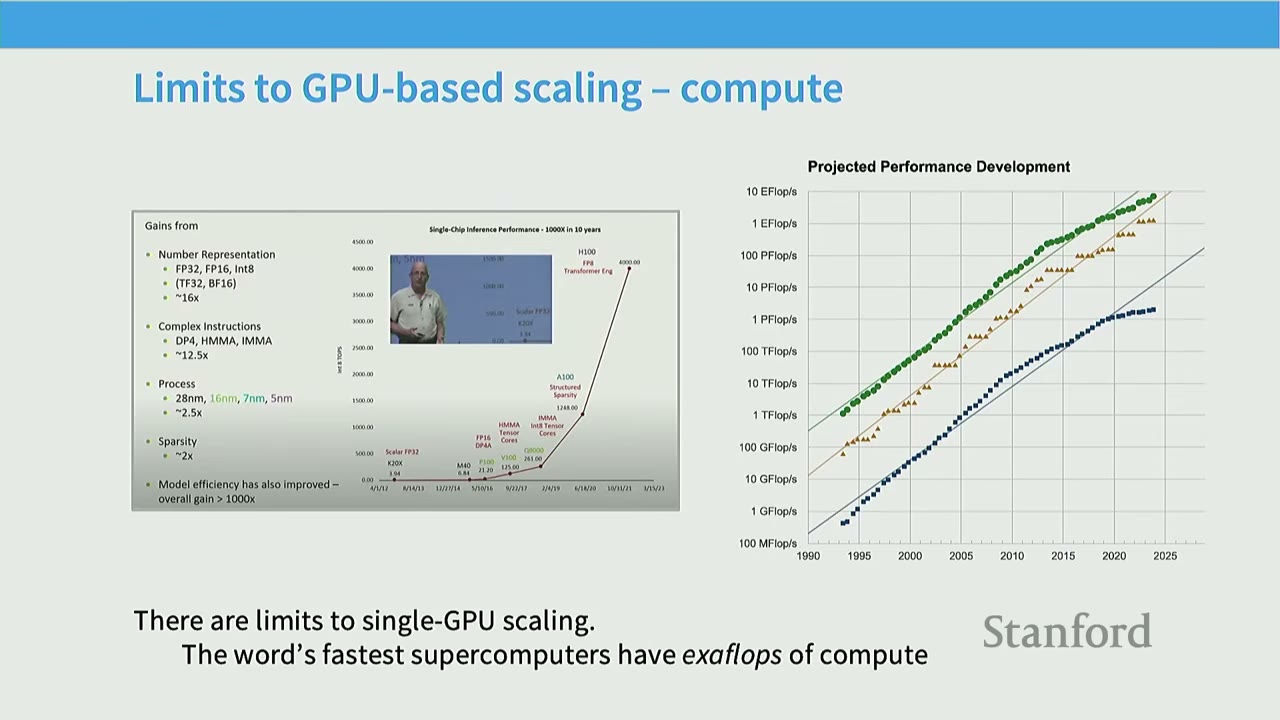
While single-GPU compute (FLOPs/GPU) has seen impressive exponential growth, training the largest LLMs today requires more than a single GPU can offer. The world's fastest supercomputers already operate at exaFLOPs of compute, indicating the need for distributed systems.
[02:43] Limits to GPU-based Scaling - Memory
Models are getting extremely large, with billions and even trillions of parameters (e.g., GPT-3 175B, Megatron-Turing NLG 530B). A single GPU often cannot fit these models into its memory. This presents both compute and memory constraints that necessitate multi-machine parallelism.
[03:24] Multi-GPU, Multi-Machine Parallelism Hardware Overview
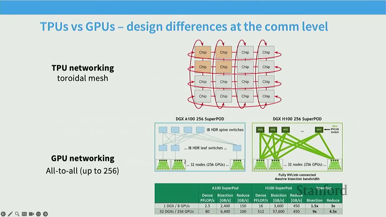
Modern GPU servers (like NVIDIA DGX systems) are designed with a hierarchy of communication speeds: * Intra-GPU parallelism (within a single machine): GPUs within the same server are connected via very high-speed interconnects (e.g., NVLink, xGMI). This allows for very fast communication between GPUs on the same node. * Inter-node parallelism (across machines): Communication between GPUs on different machines (nodes) is slower, typically going through network switches (e.g., HDR InfiniBand, PCIe Express). This creates a tiered communication latency. * TPU Networking: Google's TPUs use a toroidal mesh topology, where each chip primarily communicates with its immediate neighbors very quickly. This design is highly scalable for collective communication operations. In contrast, GPUs often use an all-to-all connection up to a certain number of GPUs (e.g., 256), beyond which communication becomes slower due to hierarchical switching.
This hardware hierarchy dictates how models are effectively parallelized in practice.
[04:57] Basics of Collective Communication
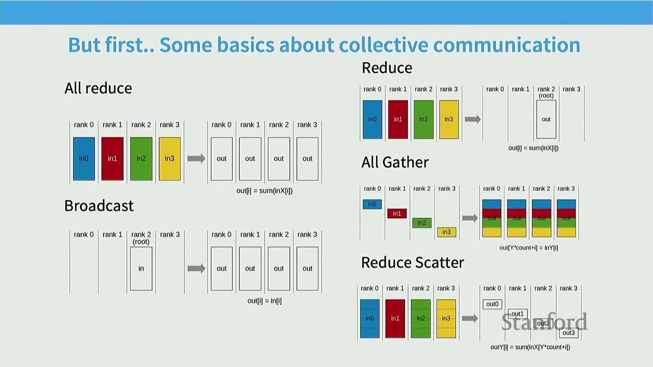
Collective communication operations are fundamental for distributed training.
* All Reduce: Each rank (GPU/machine) has an input (inX). All inputs are combined (e.g., summed), and the final result (out) is copied to all ranks. Cost is roughly 2 * size_of_data.
* Broadcast: A root rank's input (in) is copied to all other ranks' outputs (out). Cost is roughly 1 * size_of_data.
* Reduce: Similar to all_reduce, but the combined result (out) is only sent to one root rank.
* All Gather: Each rank's input (inX) is appended to form a larger output, and this full combined output is copied to all ranks.
* Reduce Scatter: Each rank's input (inX) is combined (e.g., summed) with parts of other ranks' inputs, and then a portion of the combined result is sent to each rank.
[07:03] Important Detail: all_reduce vs reduce_scatter-gather
An important equivalence: an all_reduce operation can be implemented as two steps: a reduce_scatter followed by an all_gather.
* All Reduce: All GPUs contribute their data (A, B, C, D), and all GPUs receive the sum (A+B+C+D).
* Reduce-Scatter + All-Gather:
1. Reduce-Scatter: Each GPU sums a portion of the data from all other GPUs. For example, GPU0 receives (A0+B0+C0+D0), GPU1 receives (A1+B1+C1+D1), etc. (where A0 is the first part of A, B0 is the first part of B, etc.).
2. All-Gather: Each GPU then broadcasts its combined portion to all other GPUs, so every GPU eventually reconstructs the full sum (A+B+C+D).
Key Insight: In the bandwidth-limited regime, this two-step approach (reduce_scatter + all_gather) is often the best you can do, and it has the same communication cost as a direct all_reduce. This equivalence is crucial for understanding the performance characteristics of parallelization algorithms.
[08:32] TPUs vs GPUs - Design Differences at the Communication Level

- TPU Networking: Uses a toroidal mesh, where chips primarily communicate with neighbors. This is highly scalable but limits direct communication to non-neighbors.
- GPU Networking: Often uses an all-to-all connection up to ~256 GPUs (within a superpod/rack) via high-bandwidth NVLink/InfiniBand. Beyond this, communication typically goes through slower leaf/spine switches.
This difference implies that for collective communications, TPUs might be more efficient for certain patterns due to their direct neighbor connections, while GPUs excel at all-to-all communication within their high-bandwidth clusters.
[10:27] Part 1 Recap
- New unit of compute: The datacenter (not just a single GPU).
- What we want from multi-machine scaling:
- Linear memory scaling: Max model parameters scales linearly with the number of GPUs.
- Linear compute scaling: Model FLOPs scale linearly with the number of GPUs.
- Simple collective comms primitives: Algorithms are built by combining these primitives, so performance analysis often boils down to counting communication operations.
[12:33] Part 2 - Standard LLM Parallelization Primitives
How do we parallelize LLMs? There are three important ideas:
- Data Parallelism (DP):
- Naive data parallel
- ZeRO levels 1-3
- Model Parallelism (MP):
- Pipeline parallel
- Tensor parallel
- Activation Parallelism:
- Sequence parallel
These techniques, when combined, provide the tools to scale both compute and memory gracefully across many machines.
[14:17] Naive Data Parallelism
Starting Point: Imagine we are doing naive Stochastic Gradient Descent (SGD). $$ \theta_{t+1} = \theta_t - \eta \nabla_B f(x_i) $$ Naive Parallelism: Split the B-sized batch across M machines. Exchange gradients to synchronize.
How does this do?
* Compute scaling: Each GPU processes B/M examples. This is good if B is large enough to saturate GPU compute.
* Communication overhead: Transmits 2 * #params every batch (for all_reduce). This is okay if batches are big, as computation can mask communication.
* Memory scaling: None. Every GPU needs #params at least (for model weights, gradients, and optimizer states).
[16:10] What's Wrong with Naive Data Parallel? - Memory
Memory is a significant problem. A single GPU often runs out of memory. In naive DP, we copy the entire model parameters to each GPU.
Memory Situation is Terrible: Depending on precision (e.g., BF16/FP32), a single parameter requires multiple bytes for different components: * 2 bytes for FP/BF16 model parameters * 2 bytes for FP/BF16 gradients * 4 bytes for FP32 master weights (the thing you accumulate into SGD) * 4 (or 2) bytes for FP32/BF16 Adam first moment estimates * 4 (or 2) bytes for FP32/BF16 Adam second moment estimates
This means we need ~5 copies of weights, totaling ~16 bytes per parameter. This quickly exhausts GPU memory, especially for large models.
[17:57] ZeRO - Solving the Memory Overhead Issue of DP
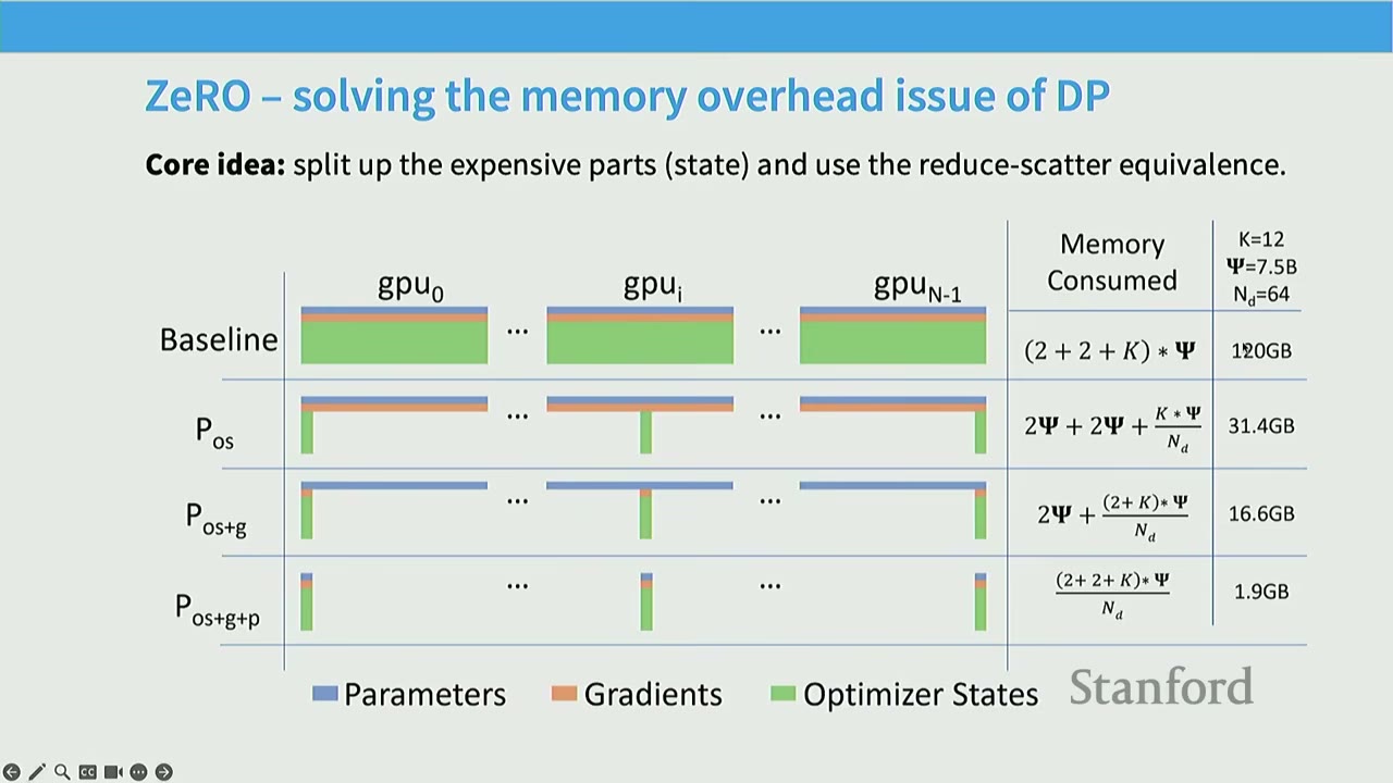
Core idea: Split up the expensive parts (state) and use the reduce-scatter equivalence.
Let's visualize memory usage for a 7.5B parameter model distributed over 64 accelerators (GPUs) with naive DP: * Baseline: Total memory consumed is ~120GB. This includes parameters (P), gradients (G), and optimizer states (OS). The optimizer states (OS) are the largest component.
ZeRO stages:
* ZeRO Stage 1 (P_os): Optimizer state sharding.
* High-level idea: Split up the optimizer state (first + second moments) across GPUs. Everyone still has the parameters and gradients. Each worker is responsible for updating a subset of parameters (corresponding to its slice).
* Memory consumed: $(2 + 2 + K) \frac{\Psi}{N_d}$ where $K$ is the optimizer state size, $\Psi$ is total parameters, $N_d$ is number of devices. This reduces memory from 120GB to ~31.4GB.
* How it works:
1. Everyone computes a full gradient on their subset of the batch.
2. ReduceScatter the gradients: Each GPU (rank) receives the sum of gradients for the parameters it owns. Communication cost: 2 * #params.
3. Each machine updates their parameter slice using their gradient + state.
4. AllGather the updated parameters: Each GPU broadcasts its updated parameter slice to all other GPUs, so everyone has the full updated model. Communication cost: 2 * #params.
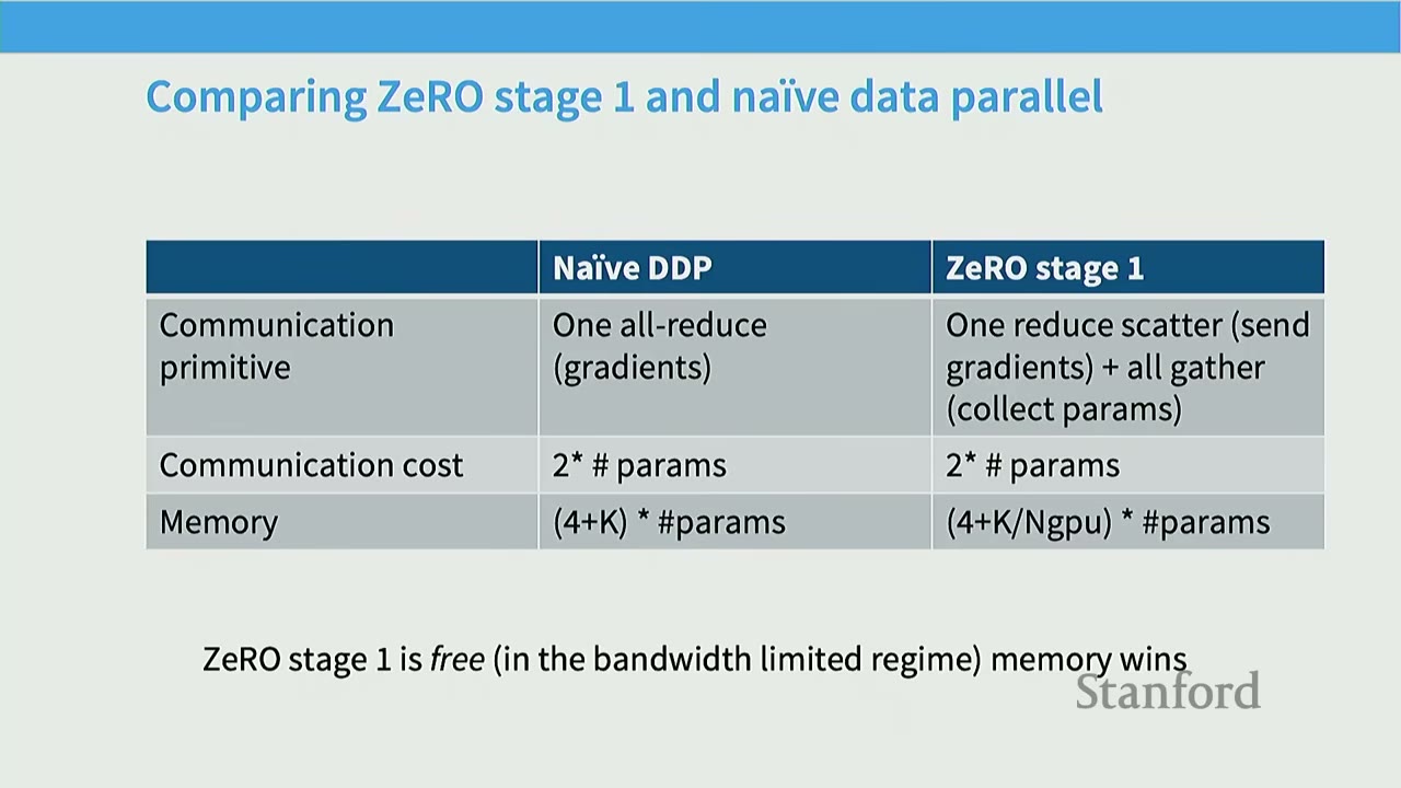
* Comparison with Naive DDP:
* Communication primitive: Naive DDP uses all_reduce (one gradient). ZeRO stage 1 uses reduce_scatter (gradients) + all_gather (parameters).
* Communication cost: Both are 2 * #params.
* Memory: Naive DDP: (4 + K) * #params. ZeRO stage 1: (4 + K/Ngpu) * #params.
* Key point: ZeRO stage 1 is free in the bandwidth-limited regime (same communication cost as all_reduce) but provides significant memory savings.
-
ZeRO Stage 2 (P_os+g): Optimizer state + gradient sharding.
- High-level idea: Also keep the gradients (pink slices) sharded across the machines.
- Memory consumed: $(2 + K) \frac{\Psi}{N_d}$. This reduces memory further to ~16.6GB.
- Complexity: We can never instantiate a full gradient vector. Each worker must compute a full gradient (since we're doing a data parallel run). This means during the backward pass, as soon as a layer's gradients are computed, they must be immediately reduced/scattered to the owning GPU and then freed. This requires incremental computation/communication.
- How it works:
- Everyone incrementally goes backward on the computation graph.
- After computing a layer's gradients, immediately
reduce_scatterthis to the right worker (the GPU owning that parameter slice). - Once gradients are not needed in the backward graph, immediately free them.
- Each machine updates their parameter using their gradient + state.
AllGatherthe parameters.
- Communication cost: Still
2 * #params(total, not per layer).
-
ZeRO Stage 3 (P_os+g+p): Optimizer state + gradient + parameter sharding (aka FSDP - Fully Sharded Data Parallel).
- High-level idea: Shard everything, including parameters. Use the same incremental communication/computation ideas. Send and request parameters on demand while stepping through the compute graph.
- Memory consumed: $(2 + K) \frac{\Psi}{N_d}$. This reduces memory further to ~1.9GB.
- How it works (baby version):
- Forward Pass: For each layer,
all_gatherthe weights needed for that layer. Perform the forward computation. Immediatelyfreethe weights. This happens incrementally layer by layer. - Backward Pass: For each layer,
all_gatherthe weights. Perform the backward computation.Reduce_scatterthe gradients to the owning GPU. Immediatelyfreethe weights and gradients. - Update Weights: Each GPU updates its owned parameter slice.
- All-Gather Parameters:
All_gatherthe updated parameters so all GPUs have the full updated model.
- Forward Pass: For each layer,
- Communication cost:
2 * all_gather(for all parameters) +1 * reduce_scatter(for all parameters). Total3 * #params. - Key point: The surprising part is that this is possible with low overhead due to overlapping communication and computation. All-gathers can happen at once while forward computation proceeds, masking the communication cost. This is achieved by queuing requests for weights/gradients before they are actually needed.
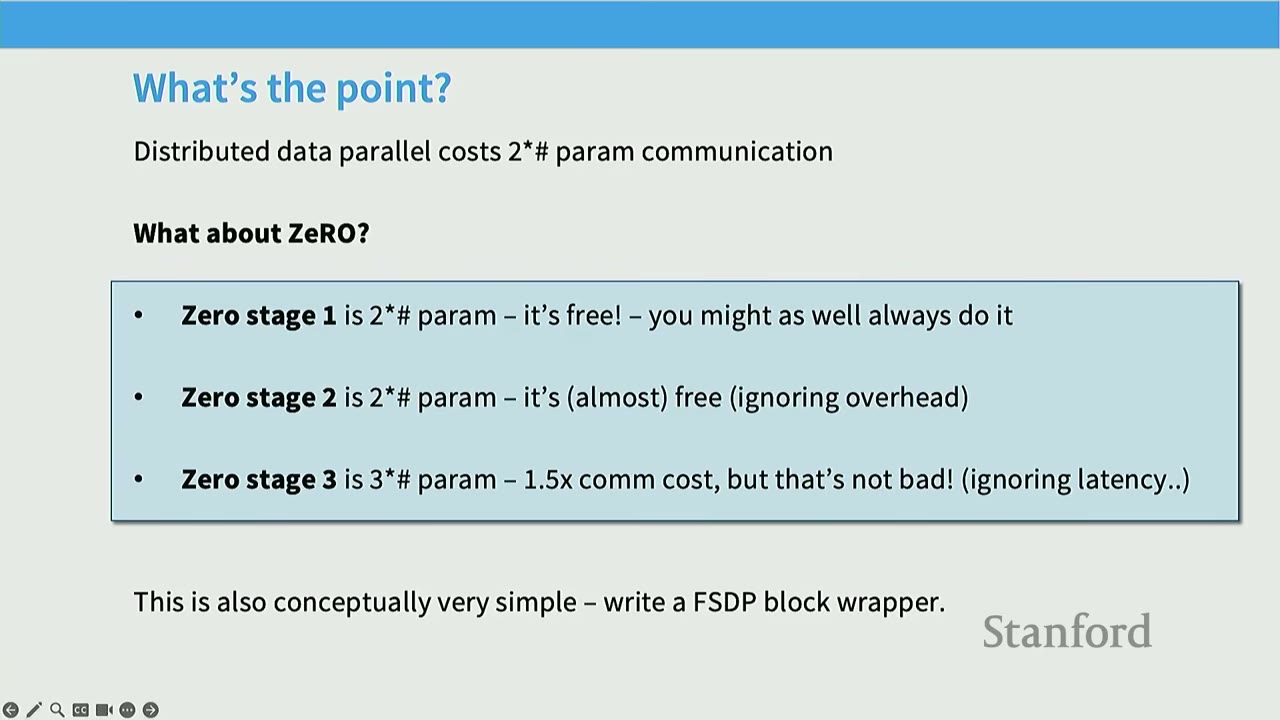
[18:28] What's the Point? (ZeRO Summary)
- Distributed data parallel costs:
2 * #paramcommunication (for naive DP). - ZeRO Stage 1:
2 * #param- it's free! (same comm cost, but memory savings). You might as well always do it. - ZeRO Stage 2:
2 * #param- almost free (ignoring overhead from incremental processing). - ZeRO Stage 3:
3 * #param- 1.5x comm cost, but that's not bad! (ignoring latency, which is masked by overlapping).
ZeRO in Practice - Will it fit? On an 8x A100 80GB node: * Baseline (Naive DP): Max model size ~6.66B parameters. Formula for B/param: 12. * ZeRO Stage 1: Max model size ~16B parameters. Formula for B/param: 5. * ZeRO Stage 2: Max model size ~24.62B parameters. Formula for B/param: 2 (param) + 10 (grad + state) / 8. * ZeRO Stage 3: Max model size ~53.33B parameters. Formula for B/param: 12/8.
ZeRO allows fitting significantly larger models into memory by sharding the model state.
[30:31] Issues Remain with Data Parallel - Compute Scaling
- With data parallel, if
#machines > batch size(and near this, communication overhead is high), efficiency drops. - There are diminishing returns to batch sizes for optimization. Beyond a "critical batch size", increasing the batch size yields little benefit for optimization.
- This means data parallel alone cannot achieve arbitrarily large parallelism. Batch size becomes a critical resource that needs to be managed.
[44:00] Issues Remain with Data Parallel - Models Don't Fit
- ZeRO stages 1 and 2 don't scale memory for activations.
- ZeRO stage 3 is good in principle but can be slow and does not reduce activation memory.
- This highlights the need for other parallelism strategies when models become too large to fit even with ZeRO.
[45:14] Beyond Data Parallel - Model Parallelism
What is Model Parallelism? * It splits the parameters across GPUs (like ZeRO3). * But it communicates activations (while ZeRO3 sends parameters).
We cover two different types of model parallelism: 1. Pipeline Parallelism (PP) 2. Tensor Parallelism (TP)
[46:09] Layer-wise Parallelism (Pipeline Parallel)
Concept: Cuts up layers, assigns some subset to GPUs. Activations and partial gradients are passed back and forth. * Example: Layer 0 on GPU0, Layer 1 on GPU1, etc. For a forward pass, GPU0 computes Layer 0, sends activations to GPU1. GPU1 computes Layer 1, sends activations to GPU2, and so on. The backward pass reverses this.
What's wrong with layer-wise parallelism?
* Terrible utilization: With N GPUs, each GPU is active 1/N of the time.
* The "Bubble": GPUs are idle most of the time, waiting for the forward pass to propagate through the pipeline and the backward pass to propagate back. This creates a large "bubble" of idle time.
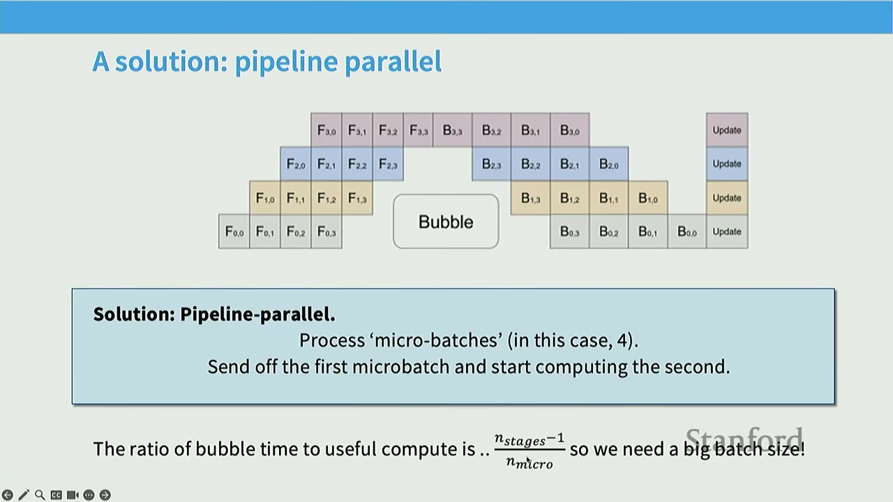
[47:54] A Solution: Pipeline Parallel (Micro-batching)
Solution: Process 'micro-batches'. * Instead of waiting for the entire batch to clear the pipeline, split the batch into smaller micro-batches. * As soon as the first micro-batch completes a stage, send its activations to the next GPU and start computing the second micro-batch on the first GPU. * This allows overlapping computation and communication, reducing the bubble size. * Ratio of bubble time to useful compute: $\frac{N_{stages} - 1}{N_{microbatches}}$. * Key point: If you have a large number of micro-batches (which means a large batch size), the bubble can be hidden, leading to better utilization. Batch size becomes a resource that can be spent to improve pipeline parallel efficiency.
[49:27] Why Pipeline Parallel?
Pipelines seem terrible due to the bubble, so why do we use them? 1. Pipelines save memory (compared to DDP): By distributing layers, each GPU only needs to store the parameters and activations for its assigned layers, not the entire model. 2. Pipelines can have good communication properties (compared to FSDP): It depends only on activations (batch_size * sequence_length * hidden_dim) and communication is point-to-point. This can be favorable on slower network links (e.g., inter-node communication across racks or data centers).
Rule of thumb: Generally, pipeline parallel is used on slower network links (i.e., inter-node) as a way to get better memory-wise scaling.
[50:48] Pipeline Performance is Highly Dependent on Batch Size
- Observation: With a small batch size (e.g., 8), increasing pipeline parallel size (number of GPUs involved in the pipeline) rapidly degrades throughput per GPU.
- Observation: With a large batch size (e.g., 128), throughput per GPU remains relatively flat even with increasing pipeline parallel size.
- Conclusion: Batch sizes are key to hiding the bubble. Otherwise, pipeline rapidly degrades performance.
[51:24] Trading Communication Bandwidth for Utilization
More complex pipeline patterns (e.g., interleaving forward and backward passes, assigning multiple stages to each device) can improve utilization, but at the cost of increased communication bandwidth.
[51:54] "Zero Bubble" Pipelining (Dualpipe)
This is an advanced technique to eliminate the bubble in pipeline parallelism. * Core Idea: Split the backward pass into two parts: 1. Backpropagating activations (computing $\frac{\partial L}{\partial z}$ and $\frac{\partial L}{\partial x}$). 2. Computing weight gradients (computing $\frac{\partial L}{\partial W}$). * The second part (computing weight gradients) can be done whenever, as it doesn't have serial dependencies on subsequent layers' activation backpropagation. * By carefully rescheduling the weight gradient computations into the idle "bubble" time, utilization can be significantly improved. * Challenge: This is extremely complicated to implement, requiring deep intervention in the autodiff system and careful scheduling.
[52:23] Model Parallel Along the Width Axes (Tensor Parallel)
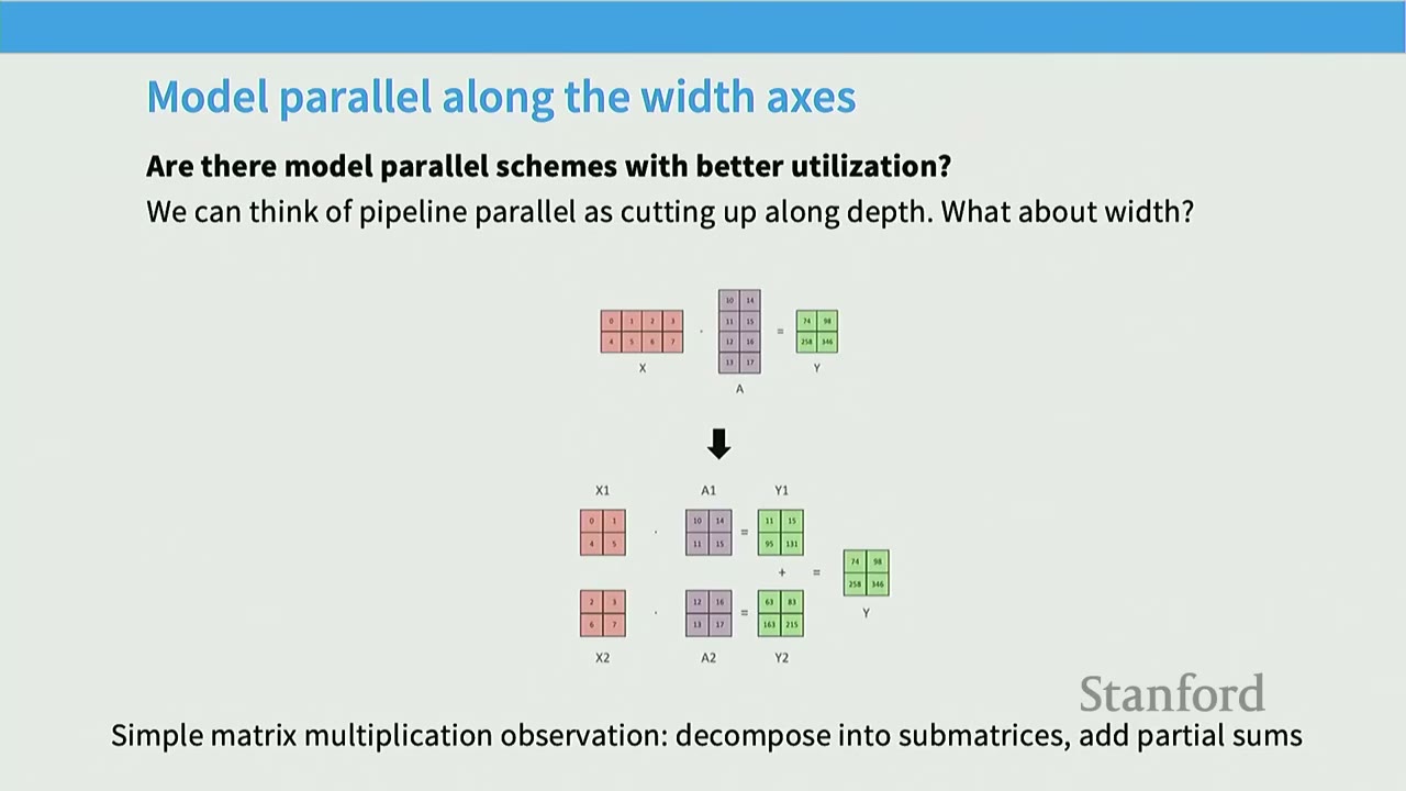
Question: Are there model parallel schemes with better utilization than pipeline parallel?
* Pipeline parallel cuts along the depth dimension (layers). What about cutting along the width dimension?
* Observation: Most of the computation in LLMs is matrix multiplies.
* Tensor Parallel Idea: Decompose large matrix multiplies into smaller submatrices that can be processed in parallel, and then combine partial sums.
* Example: For $X \times A = Y$, split $A$ into $A_1, A_2$ (columns) and $X$ into $X_1, X_2$ (rows). Then $Y = X_1 A_1 + X_2 A_2$.
* Alternatively, split $A$ into $A_1, A_2$ (rows) and $X$ into $X_1, X_2$ (columns). Then $Y = X A_1 + X A_2$.
* Implementation in LLMs (e.g., Transformer layer):
* Assign columns of weight matrices (A1, A2) and rows of weight matrices (B1, B2) to separate GPUs.
* Forward pass: Input $X$ is copied to all GPUs. Each GPU computes its part ($X A_1$ and $X A_2$). Then, an all_reduce is performed to sum the partial results (e.g., for the output of a feed-forward layer).
* Backward pass: Gradients for the output are copied to all GPUs. Each GPU computes its part of the gradient. Then, an all_reduce is performed to sum the partial gradients.
[57:50] When Do We Tensor Parallel?
- Rule of thumb: Tensor parallel is typically applied within a node (up to 8 GPUs) due to high-speed interconnects (NVLink).
- Performance: Tensor parallel is very bandwidth-hungry. While it offers memory scaling, it introduces significant communication overhead.
- Example from Hugging Face: Throughput per GPU drops by ~10-12% for TP=2 or TP=4.
- The drop becomes much steeper for higher TP values (e.g., 42.7% for TP=16, 65.6% for TP=32).
- Conclusion: Tensor parallel is often limited to the number of GPUs within a single node (e.g., 8 GPUs) to leverage the fastest available communication.
[1:00:44] Tensor Parallel - Pros and Cons vs Pipeline Parallel
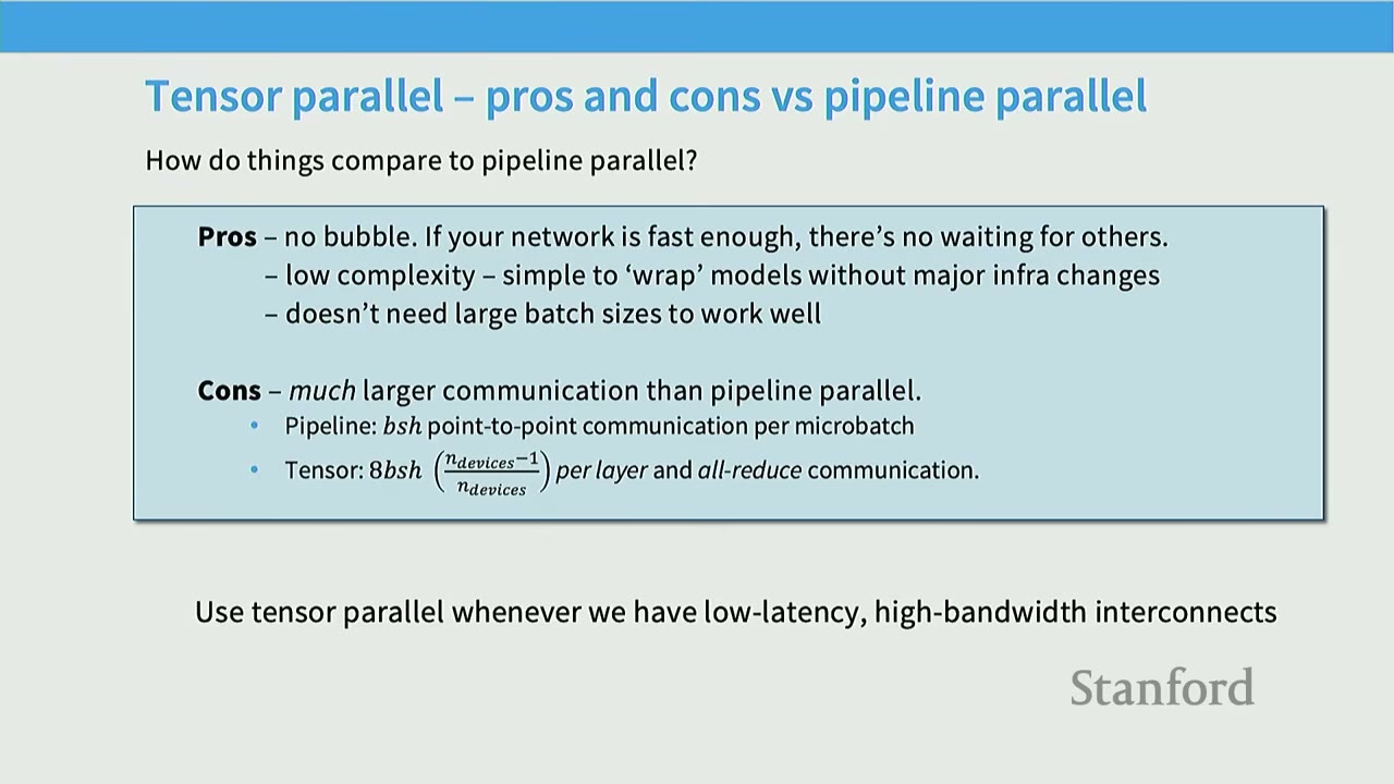
Pros of Tensor Parallel: * No bubble (unlike PP). * Low complexity: Simple to "wrap" models without major infra changes. * Doesn't need large batch sizes to work well.
Cons of Tensor Parallel: * Much larger communication than pipeline parallel. * Pipeline: Batch size * hidden_dim point-to-point communication per microbatch. * Tensor: 8 * batch_size * hidden_dim / N_devices per layer and all-reduce communication. * Rule of thumb: Use tensor parallel whenever we have low-latency, high-bandwidth interconnects (e.g., within a GPU node).
[1:03:33] A Final Complexity - Memory is Dynamic! (Activation Memory)
Memory isn't just the static bits (parameters, optimizer states), but also dynamic activations. Activations can be very large. * Observation: A memory profile of a standard forward/backward pass shows dynamic memory usage. * Parameters (static) and optimizer state (static after iteration 0) form a baseline. * Activations (red, blue) grow during the forward pass and are freed during the backward pass. * Gradients (yellow) accumulate during the backward pass. * Peak memory: The peak memory usage often occurs mid-backward pass, where some activations are still present, and gradients are accumulating.
[1:04:58] A Final Complexity - Activation Memory
- Tensor and pipeline parallel can linearly reduce parameter and optimizer state memory.
- But what about activations? Activation memory doesn't parallelize as cleanly.
- As models get bigger, activation memory (green bars) grows significantly, even with aggressive parameter/optimizer state sharding.
- Some parts of activation memory (e.g., for LayerNorm, Dropout, MLP inputs) don't parallelize well with TP/PP.
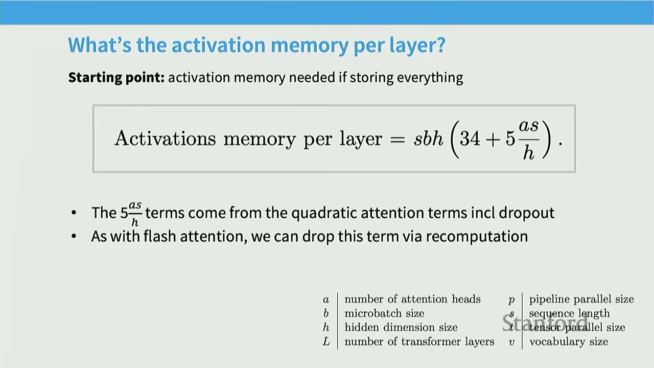
[1:05:55] What's the Activation Memory Per Layer?
For a transformer layer, the activation memory per layer (if storing everything) is:
$$ \text{activations memory per layer} = \text{sbh} \left( 34 + \frac{as}{h} + \frac{5}{h} \right) $$
Where:
* s: sequence length
* b: microbatch size
* h: hidden dimension size
* a: number of attention heads
- The $\frac{5as}{h}$ term comes from the quadratic attention terms (e.g., attention scores, values, keys) and includes dropout.
- The $34$ term comes from MLP and other pointwise operations.
- With flash attention, we can drop the $\frac{as}{h}$ term via recomputation.
[1:07:04] Activation Under Tensor Parallel
If we apply tensor parallel (splitting matrix multiplies in attention + MLP), the activation memory per layer becomes:
$$ \text{activations memory per layer} = \text{sbh} \left( 10 + \frac{24}{t} + \frac{5}{ht} \right) $$
Where t is the number of devices for tensor parallelism.
* The remaining 10 term is for LayerNorm (4sbh), Dropout (2sbh), and inputs to the attention and MLP (4sbh).
* These terms will continue to grow with size and are not divided by t. They represent pointwise operations that don't parallelize well with tensor parallel.
[1:07:59] Making Memory Truly Linear - Sequence Parallel
Observation: All the 10sbh terms (from the previous slide) are pointwise ops over the sequence.
* Idea: Split up the layer norm/dropout terms along the sequence axis. This is called Sequence Parallelism (SP).
* Forward pass: all_gather (g) is used to combine results from different sequence chunks.
* Backward pass: reduce_scatter (g') is used to combine gradients for different sequence chunks.
* In the backward pass, the two are reversed.
This allows parallelizing the remaining non-matrix multiply components of activation memory.
Putting it together to get full linear scaling for memory: By combining tensor parallel, sequence parallel, and selective activation recomputation (like Flash Attention), the activation memory per transformer layer can be reduced to: $$ \text{sbh} \left( \frac{34}{t} \right) $$ This achieves true linear scaling of activation memory with the number of devices.
[1:13:13] Recap: LLM Parallelism Table
| Strategy | Sync Overhead | Memory | Bandwidth | Batch Size | Easy to Use? |
|---|---|---|---|---|---|
| DDP/ZeRO1 | Per-batch | No scaling | 2 * #param |
Linear | Very |
| FSDP (ZeRO3) | Per-batch | Linear | 3 * #param |
Linear | Very |
| Pipeline | Per-pipeline | Linear | Activations | No Impact | NO |
| Tensor + Seq | Per-transformer block | Linear | 8 * activations per layer + all_reduce |
No Impact | YES |
Key takeaway: You have to balance limited resources: memory, bandwidth, batch size.
[1:14:57] Model vs Tensor Parallel (TPU Book)
- Key Quantity: Global batch size (divided by GPU).
- Observation: If batch size is too small (e.g., <400), no single parallelism scheme is efficient. You're communication bound.
- Observation: As batch size increases, different strategies become optimal:
- Small batch size: FSDP only.
- Medium batch size: Mixed FSDP + MP (Tensor Parallel).
- Large batch size: Both FSDP + MP and pure FSDP work well.
- Very large batch size: Pure FSDP is sufficient.
- This illustrates why you mix parallelism strategies and how batch size influences the optimal choice.
[1:16:42] "3D Parallelism" - Putting It All Together
Simple rules of thumb from the literature:
1. Until your model fits in memory:
* Use Tensor Parallel up to N_GPUs_per_machine (e.g., 8).
* Use Pipeline Parallel across machines (or ZeRO-3, depending on bandwidth).
2. Then until you run out of GPUs:
* Scale the rest of the way with Data Parallel.
* If your batch size is small, use gradient accumulation to trade batch size for better communication efficiency.
[1:18:47] Scaling Strategies from Narayanan 2021 (Megatron-LM)
This paper shows how Megatron-LM trained models from 1.7B to 1T parameters using a combination of parallelism strategies. * Tensor Parallel (TP): Starts at 1, then goes up to 8, and caps out at 8. They use TP first. * Pipeline Parallel (PP): Stays at 1 initially, but once models get big enough (can't fit), PP increases to compensate. * Data Parallel (DP): Starts as large as possible (e.g., 32), then slowly decreases as PP increases. DP is used to scale the rest of the way.
They achieve 40-52% of theoretical peak FLOPs, which is very good.
[1:20:09] Careful '3D' Parallelism Gives Linear Gains
- Careful 3D parallelism (combining TP, PP, DP) gives flat achieved TFLOPs/GPU, meaning linear scaling in total FLOPs as more GPUs are added.
- TP=8 is often optimal for throughput per GPU, even with varying batch sizes.
[1:20:48] Activation Recomputation Can Pay for Itself (via Memory)
- Activation recomputation enables larger batch sizes (by reducing activation memory).
- Larger batch sizes, in turn, improve throughput (e.g., by hiding pipeline bubbles or reducing communication overhead).
- So, even though recomputation adds FLOPs, it can pay for itself by allowing larger batches and thus better overall throughput.
[1:21:10] Recent LMs - What Do They Do?
- Dolma (7B, FSDP): Primarily uses FSDP (ZeRO3), likely intra-node.
- DeepSeek (V3 - 16B): Uses ZeRO stage 1 + Tensor Parallel + Sequence Parallel + Pipeline Parallel (16-way PP, 64-way Expert Parallel, 8-way TP).
- Yi (34B): Uses ZeRO stage 1 + Tensor Parallel + Pipeline Parallel. For MOE (Mixture of Experts) models, they use "E-lightning" which replaces TP with Expert Parallelism.
- Llama 3 405B: Uses TP=8, CP=1 (Context Parallel, for long context training), PP=16, DP=128. This is a complex network-aware parallelism configuration.
[1:23:09] Side Note - GPU Failures at This Scale!
- Training large models on thousands of GPUs for weeks/months inevitably encounters hardware failures.
- Llama 3 405B reported significant interruptions:
- Faulty GPU: 30.1%
- Faulty HBM3 Memory: 17.2%
- Software Bug: 12.9%
- Network Switch/Cable: 8.4%
- Unplanned Host Maintenance: 7.6%
- Key takeaway: Fault tolerance and robust checkpointing are crucial for large-scale distributed training. Data corruption (silent GPU failures) is an even scarier problem.
[1:24:20] Recap for the Whole Lecture
- Scaling beyond a certain point requires multi-GPU, multi-node parallelism.
- There's no single simple solution to the parallelism problem; you probably want all 3 approaches (DP, MP, AP).
- There are simple, interpretable rules of thumb for combining different forms of parallelism in practice.
Practical Takeaways
- Memory is the primary bottleneck: For large LLMs, fitting the model (parameters, optimizer states, activations) into GPU memory is the first challenge.
- ZeRO/FSDP is essential for DP: It allows data parallelism to scale memory by sharding optimizer states, gradients, and even parameters without significant communication overhead.
- Model Parallelism for huge models: When FSDP is not enough, MP (PP or TP) is needed to distribute the model itself across devices.
- TP for intra-node, PP for inter-node: Tensor Parallelism is efficient within a node due to high-bandwidth interconnects. Pipeline Parallelism is better for slower inter-node links, especially when memory saving is critical.
- Batch size is a resource: It can be used to hide communication latency in PP or to improve optimization efficiency in DP.
- Activations are a growing concern: As models and sequence lengths increase, activation memory becomes a major bottleneck, requiring techniques like Sequence Parallelism and Activation Recomputation.
- 3D/4D Parallelism is the norm: Combining DP, MP (TP/PP), and AP (SP/Recomputation) is necessary for optimal performance and memory efficiency in state-of-the-art LLM training.
- Fault tolerance is critical: Hardware failures are inevitable at scale, necessitating robust checkpointing and recovery mechanisms.
Open Questions / Things to Remember
- The choice of parallelism strategy is highly dependent on the specific hardware topology (interconnect bandwidths, latency) and model characteristics (size, depth, sequence length).
- Implementing advanced parallelism (like zero-bubble pipelining) is extremely complex and often requires deep intervention in the framework's autodiff system.
- The trade-offs between communication overhead, memory savings, and compute utilization are constant considerations.
- The "rules of thumb" provide a practical guide, but fine-tuning often involves empirical testing and profiling.
- Data corruption (silent failures) is a hidden danger in large-scale distributed systems, potentially ruining training runs without explicit errors.## TL;DR
- Training large language models (LLMs) necessitates multi-GPU and multi-node parallelism due to memory and compute limitations of single GPUs.
- Parallelism strategies are broadly categorized into Data Parallelism (DP), Model Parallelism (MP), and Activation Parallelism (AP).
- ZeRO (Zero Redundancy Optimizer) is a key DP technique that shards optimizer states, gradients, and parameters across GPUs to save memory, effectively making DP memory-scalable.
- Model Parallelism (Pipeline and Tensor) splits the model itself across devices, trading communication overhead for memory scalability.
- Activation Parallelism (Sequence Parallelism, Activation Recomputation) addresses the significant memory footprint of intermediate activations, which can become a bottleneck for very large models or long sequences.
- Effective large-scale training often combines multiple parallelism techniques (3D/4D parallelism) to balance memory, compute, and communication costs.
Key Concepts
- Multi-GPU/Multi-node Parallelism
- Collective Communication (all_reduce, reduce_scatter, all_gather, broadcast)
- Data Parallelism (DP)
- ZeRO (Zero Redundancy Optimizer) stages 1, 2, 3 (FSDP)
- Model Parallelism (MP)
- Pipeline Parallelism (PP)
- Tensor Parallelism (TP)
- Activation Parallelism
- Sequence Parallelism (SP)
- Activation Recomputation
- Batch Size as a Resource
- Communication vs. Computation Bound
- Hardware Hierarchy (NVLink, InfiniBand, Toroidal Mesh)
[00:00] Introduction: The Need for Multi-Machine Parallelism
The lecture focuses on multi-machine optimization, specifically parallelism across machines for training huge models.
Goals: * Understand the systems complexities of training huge models. * Explore different parallelization paradigms and why people use multiple approaches at once. * Describe what large-scale training runs often look like.
Outline: * Part 1: Basics of networking for LLMs. * Part 2: Different forms of parallel LLM training. * Part 3: Scaling and training big LMs with parallelism.
[00:05] Limits to GPU-based Scaling - Compute
While single-GPU compute (FLOPs/GPU) has seen impressive exponential growth, training the largest LLMs today requires more than a single GPU can offer. The world's fastest supercomputers already operate at exaFLOPs of compute, indicating the need for distributed systems.
[02:43] Limits to GPU-based Scaling - Memory
Models are getting extremely large, with billions and even trillions of parameters (e.g., GPT-3 175B, Megatron-Turing NLG 530B). A single GPU often cannot fit these models into its memory. This presents both compute and memory constraints that necessitate multi-machine parallelism.
[03:24] Multi-GPU, Multi-Machine Parallelism Hardware Overview
Modern GPU servers (like NVIDIA DGX systems) are designed with a hierarchy of communication speeds: * Intra-GPU parallelism (within a single machine): GPUs within the same server are connected via very high-speed interconnects (e.g., NVLink, xGMI). This allows for very fast communication between GPUs on the same node. * Inter-node parallelism (across machines): Communication between GPUs on different machines (nodes) is slower, typically going through network switches (e.g., HDR InfiniBand, PCIe Express). This creates a tiered communication latency. * TPU Networking: Google's TPUs use a toroidal mesh topology, where each chip primarily communicates with its immediate neighbors very quickly. This design is highly scalable but limits direct communication to non-neighbors. In contrast, GPUs often use an all-to-all connection up to a certain number of GPUs (e.g., 256), beyond which communication becomes slower due to hierarchical switching.
This hardware hierarchy dictates how models are effectively parallelized in practice.
[04:57] Basics of Collective Communication
Collective communication operations are fundamental for distributed training.
* All Reduce: Each rank (GPU/machine) has an input (inX). All inputs are combined (e.g., summed), and the final result (out) is copied to all ranks. Cost is roughly 2 * size_of_data.
* Broadcast: A root rank's input (in) is copied to all other ranks' outputs (out). Cost is roughly 1 * size_of_data.
* Reduce: Similar to all_reduce, but the combined result (out) is only sent to one root rank.
* All Gather: Each rank's input (inX) is appended to form a larger output, and this full combined output is copied to all ranks.
* Reduce Scatter: Each rank's input (inX) is combined (e.g., summed) with parts of other ranks' inputs, and then a portion of the combined result is sent to each rank.
[07:03] Important Detail: all_reduce vs reduce_scatter-gather
An important equivalence: an all_reduce operation can be implemented as two steps: a reduce_scatter followed by an all_gather.
* All Reduce: All GPUs contribute their data (A, B, C, D), and all GPUs receive the sum (A+B+C+D).
* Reduce-Scatter + All-Gather:
1. Reduce-Scatter: Each GPU sums a portion of the data from all other GPUs. For example, GPU0 receives (A0+B0+C0+D0), GPU1 receives (A1+B1+C1+D1), etc. (where A0 is the first part of A, B0 is the first part of B, etc.).
2. All-Gather: Each GPU then broadcasts its combined portion to all other GPUs, so every GPU eventually reconstructs the full sum (A+B+C+D).
Key Insight: In the bandwidth-limited regime, this two-step approach (reduce_scatter + all_gather) is often the best you can do, and it has the same communication cost as a direct all_reduce. This equivalence is crucial for understanding the performance characteristics of parallelization algorithms.
[08:32] TPUs vs GPUs - Design Differences at the Communication Level
- TPU Networking: Uses a toroidal mesh, where chips primarily communicate with neighbors. This is highly scalable but limits direct communication to non-neighbors.
- GPU Networking: Often uses an all-to-all connection up to ~256 GPUs (within a superpod/rack) via high-bandwidth NVLink/InfiniBand. Beyond this, communication typically goes through slower leaf/spine switches.
This difference implies that for collective communications, TPUs might be more efficient for certain patterns due to their direct neighbor connections, while GPUs excel at all-to-all communication within their high-bandwidth clusters.
[10:27] Part 1 Recap
- New unit of compute: The datacenter (not just a single GPU).
- What we want from multi-machine scaling:
- Linear memory scaling: Max model parameters scales linearly with the number of GPUs.
- Linear compute scaling: Model FLOPs scale linearly with the number of GPUs.
- Simple collective comms primitives: Algorithms are built by combining these primitives, so performance analysis often boils down to counting communication operations.
[12:33] Part 2 - Standard LLM Parallelization Primitives
How do we parallelize LLMs? There are three important ideas:
- Data Parallelism (DP):
- Naive data parallel
- ZeRO levels 1-3
- Model Parallelism (MP):
- Pipeline parallel
- Tensor parallel
- Activation Parallelism:
- Sequence parallel
These techniques, when combined, provide the tools to scale both compute and memory gracefully across many machines.
[14:17] Naive Data Parallelism
Starting Point: Imagine we are doing naive Stochastic Gradient Descent (SGD). $$ \theta_{t+1} = \theta_t - \eta \nabla_B f(x_i) $$ Naive Parallelism: Split the B-sized batch across M machines. Exchange gradients to synchronize.
How does this do?
* Compute scaling: Each GPU processes B/M examples. This is good if B is large enough to saturate GPU compute.
* Communication overhead: Transmits 2 * #params every batch (for all_reduce). This is okay if batches are big, as computation can mask communication.
* Memory scaling: None. Every GPU needs #params at least (for model weights, gradients, and optimizer states).
[16:10] What's Wrong with Naive Data Parallel? - Memory
Memory is a significant problem. A single GPU often runs out of memory. In naive DP, we copy the entire model parameters to each GPU.
Memory Situation is Terrible: Depending on precision (e.g., BF16/FP32), a single parameter requires multiple bytes for different components: * 2 bytes for FP/BF16 model parameters * 2 bytes for FP/BF16 gradients * 4 bytes for FP32 master weights (the thing you accumulate into SGD) * 4 (or 2) bytes for FP32/BF16 Adam first moment estimates * 4 (or 2) bytes for FP32/BF16 Adam second moment estimates
This means we need ~5 copies of weights, totaling ~16 bytes per parameter. This quickly exhausts GPU memory, especially for large models.
[17:57] ZeRO - Solving the Memory Overhead Issue of DP
Core idea: Split up the expensive parts (state) and use the reduce-scatter equivalence.
Let's visualize memory usage for a 7.5B parameter model distributed over 64 accelerators (GPUs) with naive DP: * Baseline: Total memory consumed is ~120GB. This includes parameters (P), gradients (G), and optimizer states (OS). The optimizer states (OS) are the largest component.
ZeRO stages:
* ZeRO Stage 1 (P_os): Optimizer state sharding.
* High-level idea: Split up the optimizer state (first + second moments) across GPUs. Everyone still has the parameters and gradients. Each worker is responsible for updating a subset of parameters (corresponding to its slice).
* Memory consumed: $(2 + 2 + K) \frac{\Psi}{N_d}$ where $K$ is the optimizer state size, $\Psi$ is total parameters, $N_d$ is number of devices. This reduces memory from 120GB to ~31.4GB.
* How it works:
1. Everyone computes a full gradient on their subset of the batch.
2. ReduceScatter the gradients: Each GPU (rank) receives the sum of gradients for the parameters it owns. Communication cost: 2 * #params.
3. Each machine updates their parameter slice using their gradient + state.
4. AllGather the updated parameters: Each GPU broadcasts its updated parameter slice to all other GPUs, so everyone has the full updated model. Communication cost: 2 * #params.
* Comparison with Naive DDP:
* Communication primitive: Naive DDP uses all_reduce (one gradient). ZeRO stage 1 uses reduce_scatter (gradients) + all_gather (parameters).
* Communication cost: Both are 2 * #params.
* Memory: Naive DDP: (4 + K) * #params. ZeRO stage 1: (4 + K/Ngpu) * #params.
* Key point: ZeRO stage 1 is free in the bandwidth-limited regime (same communication cost as all_reduce) but provides significant memory savings.
-
ZeRO Stage 2 (P_os+g): Optimizer state + gradient sharding.
- High-level idea: Also keep the gradients (pink slices) sharded across the machines.
- Memory consumed: $(2 + K) \frac{\Psi}{N_d}$. This reduces memory further to ~16.6GB.
- Complexity: We can never instantiate a full gradient vector. Each worker must compute a full gradient (since we're doing a data parallel run). This means during the backward pass, as soon as a layer's gradients are computed, they must be immediately reduced/scattered to the owning GPU and then freed. This requires incremental computation/communication.
- How it works:
- Everyone incrementally goes backward on the computation graph.
- After computing a layer's gradients, immediately
reduce_scatterthis to the right worker (the GPU owning that parameter slice). - Once gradients are not needed in the backward graph, immediately free them.
- Each machine updates their parameter using their gradient + state.
AllGatherthe parameters.
- Communication cost: Still
2 * #params(total, not per layer).
-
ZeRO Stage 3 (P_os+g+p): Optimizer state + gradient + parameter sharding (aka FSDP - Fully Sharded Data Parallel).
- High-level idea: Shard everything, including parameters. Use the same incremental communication/computation ideas. Send and request parameters on demand while stepping through the compute graph.
- Memory consumed: $(2 + K) \frac{\Psi}{N_d}$. This reduces memory further to ~1.9GB.
- How it works (baby version):
- Forward Pass: For each layer,
all_gatherthe weights needed for that layer. Perform the forward computation. Immediatelyfreethe weights. This happens incrementally layer by layer. - Backward Pass: For each layer,
all_gatherthe weights. Perform the backward computation.Reduce_scatterthe gradients to the owning GPU. Immediatelyfreethe weights and gradients. - Update Weights: Each GPU updates its owned parameter slice.
- All-Gather Parameters:
All_gatherthe updated parameters so all GPUs have the full updated model.
- Forward Pass: For each layer,
- Communication cost:
2 * all_gather(for all parameters) +1 * reduce_scatter(for all parameters). Total3 * #params. - Key point: The surprising part is that this is possible with low overhead due to overlapping communication and computation. All-gathers can happen at once while forward computation proceeds, masking the communication cost. This is achieved by queuing requests for weights/gradients before they are actually needed.
[18:28] What's the Point? (ZeRO Summary)
- Distributed data parallel costs:
2 * #paramcommunication (for naive DP). - ZeRO Stage 1:
2 * #param- it's free! (same comm cost, but memory savings). You might as well always do it. - ZeRO Stage 2:
2 * #param- almost free (ignoring overhead from incremental processing). - ZeRO Stage 3:
3 * #param- 1.5x comm cost, but that's not bad! (ignoring latency, which is masked by overlapping).
ZeRO in Practice - Will it fit? On an 8x A100 80GB node: * Baseline (Naive DP): Max model size ~6.66B parameters. Formula for B/param: 12. * ZeRO Stage 1: Max model size ~16B parameters. Formula for B/param: 5. * ZeRO Stage 2: Max model size ~24.62B parameters. Formula for B/param: 2 (param) + 10 (grad + state) / 8. * ZeRO Stage 3: Max model size ~53.33B parameters. Formula for B/param: 12/8.
ZeRO allows fitting significantly larger models into memory by sharding the model state.
[30:31] Issues Remain with Data Parallel - Compute Scaling
- With data parallel, if
#machines > batch size(and near this, communication overhead is high), efficiency drops. - There are diminishing returns to batch sizes for optimization. Beyond a "critical batch size", increasing the batch size yields little benefit for optimization.
- This means data parallel alone cannot achieve arbitrarily large parallelism. Batch size becomes a critical resource that needs to be managed.
[44:00] Issues Remain with Data Parallel - Models Don't Fit
- ZeRO stages 1 and 2 don't scale memory for activations.
- ZeRO stage 3 is good in principle but can be slow and does not reduce activation memory.
- This highlights the need for other parallelism strategies when models become too large to fit even with ZeRO.
[45:14] Beyond Data Parallel - Model Parallelism
What is Model Parallelism? * It splits the parameters across GPUs (like ZeRO3). * But it communicates activations (while ZeRO3 sends parameters).
We cover two different types of model parallelism: 1. Pipeline Parallelism (PP) 2. Tensor Parallelism (TP)
[46:09] Layer-wise Parallelism (Pipeline Parallel)
Concept: Cuts up layers, assigns some subset to GPUs. Activations and partial gradients are passed back and forth. * Example: Layer 0 on GPU0, Layer 1 on GPU1, etc. For a forward pass, GPU0 computes Layer 0, sends activations to GPU1. GPU1 computes Layer 1, sends activations to GPU2, and so on. The backward pass reverses this.
What's wrong with layer-wise parallelism?
* Terrible utilization: With N GPUs, each GPU is active 1/N of the time.
* The "Bubble": GPUs are idle most of the time, waiting for the forward pass to propagate through the pipeline and the backward pass to propagate back. This creates a large "bubble" of idle time.
[47:54] A Solution: Pipeline Parallel (Micro-batching)
Solution: Process 'micro-batches'. * Instead of waiting for the entire batch to clear the pipeline, split the batch into smaller micro-batches. * As soon as the first micro-batch completes a stage, send its activations to the next GPU and start computing the second micro-batch on the first GPU. * This allows overlapping computation and communication, reducing the bubble size. * Ratio of bubble time to useful compute: $\frac{N_{stages} - 1}{N_{microbatches}}$. * Key point: If you have a large number of micro-batches (which means a large batch size), the bubble can be hidden, leading to better utilization. Batch size becomes a resource that can be spent to improve pipeline parallel efficiency.
[49:27] Why Pipeline Parallel?
Pipelines seem terrible due to the bubble, so why do we use them? 1. Pipelines save memory (compared to DDP): By distributing layers, each GPU only needs to store the parameters and activations for its assigned layers, not the entire model. 2. Pipelines can have good communication properties (compared to FSDP): It depends only on activations (batch_size * sequence_length * hidden_dim) and communication is point-to-point. This can be favorable on slower network links (e.g., inter-node communication across racks or data centers).
Rule of thumb: Generally, pipeline parallel is used on slower network links (i.e., inter-node) as a way to get better memory-wise scaling.
[50:48] Pipeline Performance is Highly Dependent on Batch Size
- Observation: With a small batch size (e.g., 8), increasing pipeline parallel size (number of GPUs involved in the pipeline) rapidly degrades throughput per GPU.
- Observation: With a large batch size (e.g., 128), throughput per GPU remains relatively flat even with increasing pipeline parallel size.
- Conclusion: Batch sizes are key to hiding the bubble. Otherwise, pipeline rapidly degrades performance.
[51:24] Trading Communication Bandwidth for Utilization
More complex pipeline patterns (e.g., interleaving forward and backward passes, assigning multiple stages to each device) can improve utilization, but at the cost of increased communication bandwidth.
[51:54] "Zero Bubble" Pipelining (Dualpipe)
This is an advanced technique to eliminate the bubble in pipeline parallelism. * Core Idea: Split the backward pass into two parts: 1. Backpropagating activations (computing $\frac{\partial L}{\partial z}$ and $\frac{\partial L}{\partial x}$). 2. Computing weight gradients (computing $\frac{\partial L}{\partial W}$). * The second part (computing weight gradients) can be done whenever, as it doesn't have serial dependencies on subsequent layers' activation backpropagation. * By carefully rescheduling the weight gradient computations into the idle "bubble" time, utilization can be significantly improved. * Challenge: This is extremely complex to implement, requiring deep intervention in the autodiff system and careful scheduling.
[52:23] Model Parallel Along the Width Axes (Tensor Parallel)
Question: Are there model parallel schemes with better utilization than pipeline parallel?
* Pipeline parallel cuts along the depth dimension (layers). What about cutting along the width dimension?
* Observation: Most of the computation in LLMs is matrix multiplies.
* Tensor Parallel Idea: Decompose large matrix multiplies into smaller submatrices that can be processed in parallel, and then combine partial sums.
* Example: For $X \times A = Y$, split $A$ into $A_1, A_2$ (columns) and $X$ into $X_1, X_2$ (rows). Then $Y = X_1 A_1 + X_2 A_2$.
* Alternatively, split $A$ into $A_1, A_2$ (rows) and $X$ into $X_1, X_2$ (columns). Then $Y = X A_1 + X A_2$.
* Implementation in LLMs (e.g., Transformer layer):
* Assign columns of weight matrices (A1, A2) and rows of weight matrices (B1, B2) to separate GPUs.
* Forward pass: Input $X$ is copied to all GPUs. Each GPU computes its part ($X A_1$ and $X A_2$). Then, an all_reduce is performed to sum the partial results (e.g., for the output of a feed-forward layer).
* Backward pass: Gradients for the output are copied to all GPUs. Each GPU computes its part of the gradient. Then, an all_reduce is performed to sum the partial gradients.
[57:50] When Do We Tensor Parallel?
- Rule of thumb: Tensor parallel is typically applied within a node (up to 8 GPUs) due to high-speed interconnects (NVLink).
- Performance: Tensor parallel is very bandwidth-hungry. While it offers memory scaling, it introduces significant communication overhead.
- Example from Hugging Face: Throughput per GPU drops by ~10-12% for TP=2 or TP=4.
- The drop becomes much steeper for higher TP values (e.g., 42.7% for TP=16, 65.6% for TP=32).
- Conclusion: Tensor parallel is often limited to the number of GPUs within a single node (e.g., 8 GPUs) to leverage the fastest available communication.
[1:00:44] Tensor Parallel - Pros and Cons vs Pipeline Parallel
Pros of Tensor Parallel: * No bubble (unlike PP). * Low complexity: Simple to "wrap" models without major infra changes. * Doesn't need large batch sizes to work well.
Cons of Tensor Parallel: * Much larger communication than pipeline parallel. * Pipeline: Batch size * sequence_length * hidden_dim point-to-point communication per microbatch. * Tensor: 8 * batch_size * hidden_dim / N_devices per layer and all-reduce communication. * Rule of thumb: Use tensor parallel whenever we have low-latency, high-bandwidth interconnects (e.g., within a GPU node).
[1:03:33] A Final Complexity - Memory is Dynamic! (Activation Memory)
Memory isn't just the static bits (parameters, optimizer states), but also dynamic activations. Activations can be very large. * Observation: A memory profile of a standard forward/backward pass shows dynamic memory usage. * Parameters (static) and optimizer state (static after iteration 0) form a baseline. * Activations (red, blue) grow during the forward pass and are freed during the backward pass. * Gradients (yellow) accumulate during the backward pass. * Peak memory: The peak memory usage often occurs mid-backward pass, where some activations are still present, and gradients are accumulating.
[1:04:58] A Final Complexity - Activation Memory
- Tensor and pipeline parallel can linearly reduce parameter and optimizer state memory.
- But what about activations? Activation memory doesn't parallelize as cleanly.
- As models get bigger, activation memory (green bars) grows significantly, even with aggressive parameter/optimizer state sharding.
- Some parts of activation memory (e.g., for LayerNorm, Dropout, MLP inputs) don't parallelize well with TP/PP.
[1:05:55] What's the Activation Memory Per Layer?
For a transformer layer, the activation memory per layer (if storing everything) is:
$$ \text{activations memory per layer} = \text{sbh} \left( 34 + \frac{as}{h} + \frac{5}{h} \right) $$
Where:
* s: sequence length
* b: microbatch size
* h: hidden dimension size
* a: number of attention heads
- The $\frac{5as}{h}$ term comes from the quadratic attention terms (e.g., attention scores, values, keys) and includes dropout.
- The $34$ term comes from MLP and other pointwise operations.
- With flash attention, we can drop the $\frac{as}{h}$ term via recomputation.
[1:07:04] Activation Under Tensor Parallel
If we apply tensor parallel (splitting matrix multiplies in attention + MLP), the activation memory per layer becomes:
$$ \text{activations memory per layer} = \text{sbh} \left( 10 + \frac{24}{t} + \frac{5}{ht} \right) $$
Where t is the number of devices for tensor parallelism.
* The remaining 10 term is for LayerNorm (4sbh), Dropout (2sbh), and inputs to the attention and MLP (4sbh).
* These terms will continue to grow with size and are not divided by t. They represent pointwise operations that don't parallelize well with tensor parallel.
[1:07:59] Making Memory Truly Linear - Sequence Parallel
Observation: All the 10sbh terms (from the previous slide) are pointwise ops over the sequence.
* Idea: Split up the layer norm/dropout terms along the sequence axis. This is called Sequence Parallelism (SP).
* Forward pass: all_gather (g) is used to combine results from different sequence chunks.
* Backward pass: reduce_scatter (g') is used to combine gradients for different sequence chunks.
* In the backward pass, the two are reversed.
This allows parallelizing the remaining non-matrix multiply components of activation memory.
Putting it together to get full linear scaling for memory: By combining tensor parallel, sequence parallel, and selective activation recomputation (like Flash Attention), the activation memory per transformer layer can be reduced to: $$ \text{sbh} \left( \frac{34}{t} \right) $$ This achieves true linear scaling of activation memory with the number of devices.
[1:13:13] Recap: LLM Parallelism Table
| Strategy | Sync Overhead | Memory | Bandwidth | Batch Size | Easy to Use? |
|---|---|---|---|---|---|
| DDP/ZeRO1 | Per-batch | No scaling | 2 * #param |
Linear | Very |
| FSDP (ZeRO3) | Per-batch | Linear | 3 * #param |
Linear | Very |
| Pipeline | Per-pipeline | Linear | Activations | No Impact | NO |
| Tensor + Seq | Per-transformer block | Linear | 8 * activations per layer + all_reduce |
No Impact | YES |
Key takeaway: You have to balance limited resources: memory, bandwidth, batch size.
[1:14:57] Model vs Tensor Parallel (TPU Book)
- Key Quantity: Global batch size (divided by GPU).
- Observation: If batch size is too small (e.g., <400), no single parallelism scheme is efficient. You're communication bound.
- Observation: As batch size increases, different strategies become optimal:
- Small batch size: FSDP only.
- Medium batch size: Mixed FSDP + MP (Tensor Parallel).
- Large batch size: Both FSDP + MP and pure FSDP work well.
- Very large batch size: Pure FSDP is sufficient.
- This illustrates why you mix parallelism strategies and how batch size influences the optimal choice.
[1:16:42] "3D Parallelism" - Putting It All Together
Simple rules of thumb from the literature:
1. Until your model fits in memory:
* Use Tensor Parallel up to N_GPUs_per_machine (e.g., 8).
* Use Pipeline Parallel across machines (or ZeRO-3, depending on bandwidth).
2. Then until you run out of GPUs:
* Scale the rest of the way with Data Parallel.
* If your batch size is small, use gradient accumulation to trade batch size for better communication efficiency.
[1:18:47] Scaling Strategies from Narayanan 2021 (Megatron-LM)
This paper shows how Megatron-LM trained models from 1.7B to 1T parameters using a combination of parallelism strategies. * Tensor Parallel (TP): Starts at 1, then goes up to 8, and caps out at 8. They use TP first. * Pipeline Parallel (PP): Stays at 1 initially, but once models get big enough (can't fit), PP increases to compensate. * Data Parallel (DP): Starts as large as possible (e.g., 32), then slowly decreases as PP increases. DP is used to scale the rest of the way.
They achieve 40-52% of theoretical peak FLOPs, which is very good.
[1:20:09] Careful '3D' Parallelism Gives Linear Gains
- Careful 3D parallelism (combining TP, PP, DP) gives flat achieved TFLOPs/GPU, meaning linear scaling in total FLOPs as more GPUs are added.
- TP=8 is often optimal for throughput per GPU, even with varying batch sizes.
[1:20:48] Activation Recomputation Can Pay for Itself (via Memory)
- Activation recomputation enables larger batch sizes (by reducing activation memory).
- Larger batch sizes, in turn, improve throughput (e.g., by hiding pipeline bubbles or reducing communication overhead).
- So, even though recomputation adds FLOPs, it can pay for itself by allowing larger batches and thus better overall throughput.
[1:21:10] Recent LMs - What Do They Do?
- Dolma (7B, FSDP): Primarily uses FSDP (ZeRO3), likely intra-node.
- DeepSeek (V3 - 16B): Uses ZeRO stage 1 + Tensor Parallel + Sequence Parallel + Pipeline Parallel (16-way PP, 64-way Expert Parallel, 8-way TP).
- Yi (34B): Uses ZeRO stage 1 + Tensor Parallel + Pipeline Parallel. For MOE (Mixture of Experts) models, they use "E-lightning" which replaces TP with Expert Parallelism.
- Llama 3 405B: Uses TP=8, CP=1 (Context Parallel, for long context training), PP=16, DP=128. This is a complex network-aware parallelism configuration.
[1:23:09] Side Note - GPU Failures at This Scale!
- Training large models on thousands of GPUs for weeks/months inevitably encounters hardware failures.
- Llama 3 405B reported significant interruptions:
- Faulty GPU: 30.1%
- Faulty HBM3 Memory: 17.2%
- Software Bug: 12.9%
- Network Switch/Cable: 8.4%
- Unplanned Host Maintenance: 7.6%
- Key takeaway: Fault tolerance and robust checkpointing are crucial for large-scale distributed training. Data corruption (silent GPU failures) is an even scarier problem.
[1:23:47] Gemma 2
- Gemma 2 (9B, 27B): Uses ZeRO3 + Model Parallelism + Data Parallelism. For TPUs, they leverage the TPUv4 and TPUv5p models. They use 512-way data replication and 1-way sharding. The optimizer state is further sharded using techniques similar to ZeRO-3.
[1:24:20] Recap for the Whole Lecture
- Scaling beyond a certain point is going to require multi-GPU, multi-node parallelism.
- There's no single simple solution to the parallelism problem; you probably want all 3 approaches (DP, MP, AP).
- There are simple and interpretable rules of thumb for combining different forms of parallelism in practice.
Practical Takeaways
- Memory is the primary bottleneck: For large LLMs, fitting the model (parameters, optimizer states, activations) into GPU memory is the first challenge.
- ZeRO/FSDP is essential for DP: It allows data parallelism to scale memory by sharding optimizer states, gradients, and even parameters without significant communication overhead.
- Model Parallelism for huge models: When FSDP is not enough, MP (PP or TP) is needed to distribute the model itself across devices.
- TP for intra-node, PP for inter-node: Tensor Parallelism is efficient within a node due to high-bandwidth interconnects. Pipeline Parallelism is better for slower inter-node links, especially when memory saving is critical.
- Batch size is a resource: It can be used to hide communication latency in PP or to improve optimization efficiency in DP.
- Activations are a growing concern: As models and sequence lengths increase, activation memory becomes a major bottleneck, requiring techniques like Sequence Parallelism and Activation Recomputation.
- 3D/4D Parallelism is the norm: Combining DP, MP (TP/PP), and AP (SP/Recomputation) is necessary for optimal performance and memory efficiency in state-of-the-art LLM training.
- Fault tolerance is critical: Hardware failures are inevitable at scale, necessitating robust checkpointing and recovery mechanisms.
Open Questions / Things to Remember
- The choice of parallelism strategy is highly dependent on the specific hardware topology (interconnect bandwidths, latency) and model characteristics (size, depth, sequence length).
- Implementing advanced parallelism (like zero-bubble pipelining) is extremely complex and often requires deep intervention in the framework's autodiff system.
- The trade-offs between communication overhead, memory savings, and compute utilization are constant considerations.
- The "rules of thumb" provide a practical guide, but fine-tuning often involves empirical testing and profiling.
- Data corruption (silent failures) is a hidden danger in large-scale distributed systems, potentially ruining training runs without explicit errors.